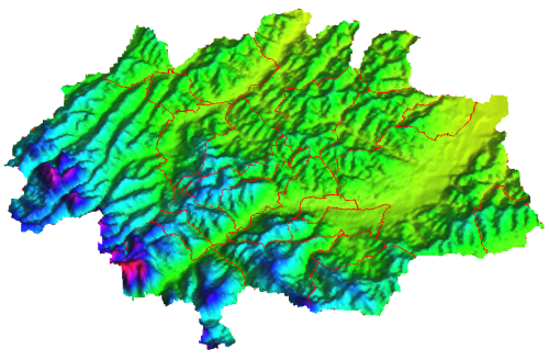
The space dimension in the decision LP matrix
A great difference with AgriPoliS is that the MIP is spatially explicit. So it will be composed of the following activities:
 spacial explicit activities *
  plot numbers
 spacial explicit investments *
  suitable plots
 other spacial implicit activities
 other spacial implicit investments
The spacial explicitness has the disadvantage of a much larger matrix, especially in case of farmers with many plots, but it has the following advantages:
- transport costs are associated directly with the individual pixels and already included in the Gross Margin;
- pixel heterogeneity (e.g. different slopes) can be included straightforward, just changing the gross margins;
- an explicit map of the region can be draw to show the different productions
- binds on individual pixels can be easily inserted on the map (e.g. if the plot_4 is already employed for perennial crops, the matrix will not have the activity option “maize on plot_4” till the perennial crop investment will dead).
An example of matrix following such approach is given:
| Resources | Prod. activity 1 on plot1 | Prod. activity 1 on plot2 | Prod. activity 1 on plot3 | Prod. activity 2 on plot1 | Prod. activity 2 on plot2 | Prod. activity 2 on plot3 | Inv. activity 3 on plot3 | Used recourses | Available resources | ||
|---|---|---|---|---|---|---|---|---|---|---|---|
| Gross margin | 300 | 295 | 305 | 60 | 58 | 62 | 140 | ||||
| … | |||||||||||
| Plot1 | 1 | 1 | 0 | 1 | |||||||
| Plot2 | 1 | 1 | 0 | 1 | |||||||
| Plot3 | 1 | 1 | 1 | 0 | 1 | ||||||
| … | |||||||||||
| Other resources | … | … | … | … | … | … | … | … | … | ||
| … | |||||||||||
| Quantities | 0 | 0 | 0 | 0 | 0 | 0 | 0 |
Gross margin already take into account that plot1 is closer than plot2 and that plot3 is even more close to the farm.
If the farmer decide to invest activity3 (a perennial crop) on plot3, the following years, “Prod. activity 1 on plot3” and “Prod. activity 2 on plot3” will obviously not be available.
This appoach let us fully differentiate between plots, e.g. on their elevation or even on their slope or exposure.
